x=rnorm(50) # Generate a vector of 50 numbers using the rnorm() functiony=x+rnorm(50,mean=50,sd=.1) # What does rnorm(50,mean=50,sd=.1) generate?cor(x,y) # Correlation of x and y
[1] 0.9949607
set.seed(1303) # Set the seed for Random Number Generator (RNG) to generate values that are reproducible.rnorm(50)
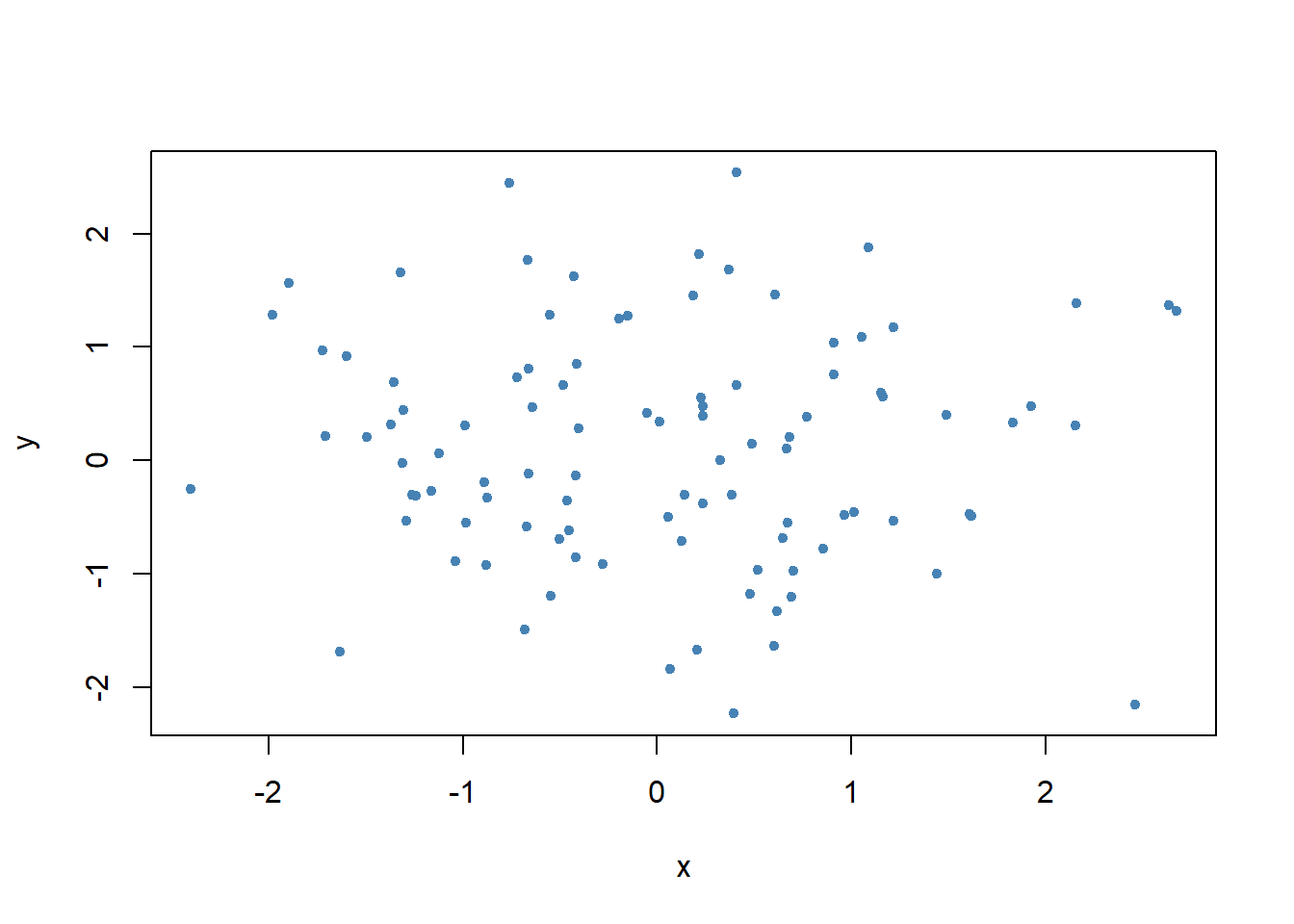
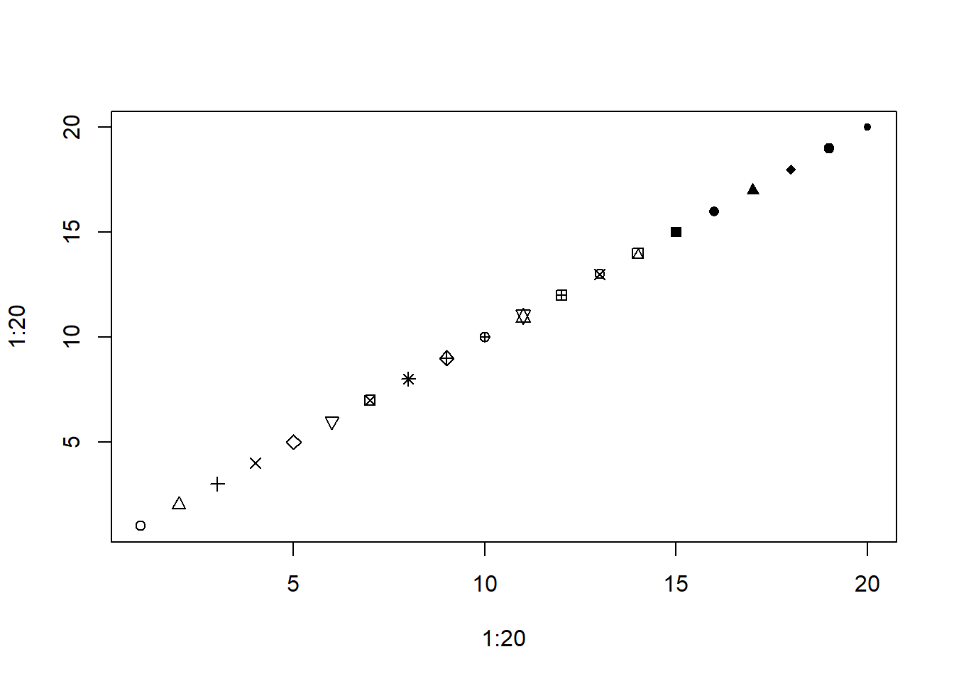
x=rnorm(100)y=rnorm(100)plot(x,y, pch=20, col ="steelblue") # Scatterplot for two numeric variables by default
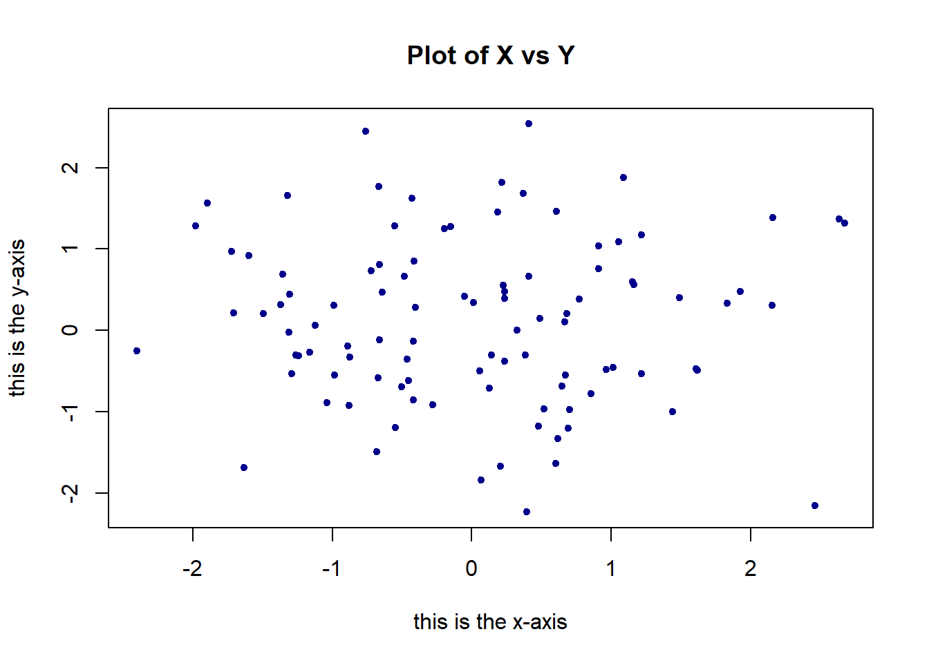
plot(x,y, pch=20, col ="darkblue",xlab="this is the x-axis",ylab="this is the y-axis",main="Plot of X vs Y") # Add labels
pdf("Figure01.pdf") # Save as pdf, add a path or it will be stored on the project directoryplot(x,y,pch=20, col="lightgreen") # Try different colors?dev.off() # Close the file using the dev.off function
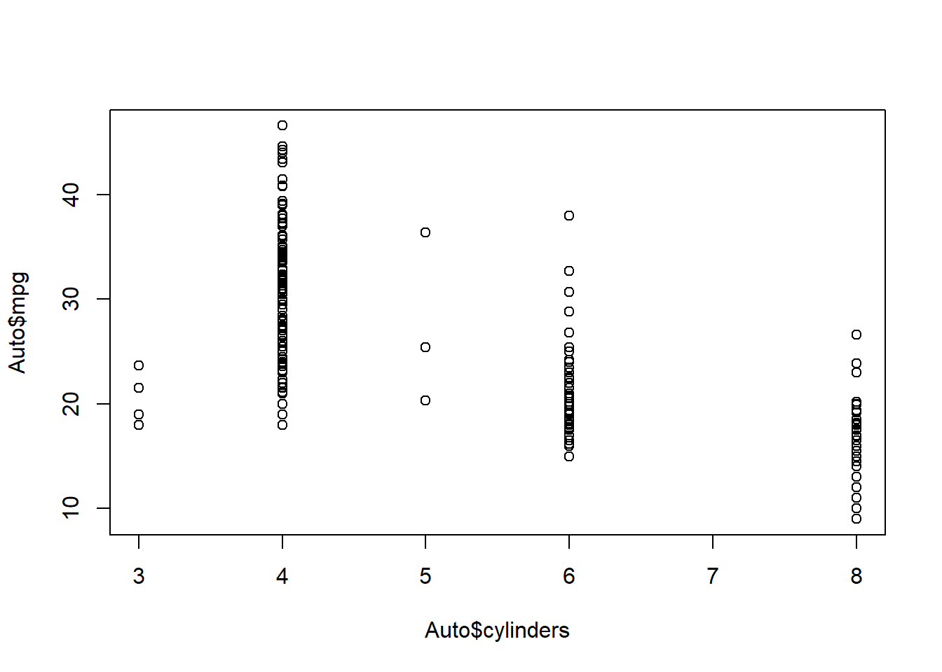
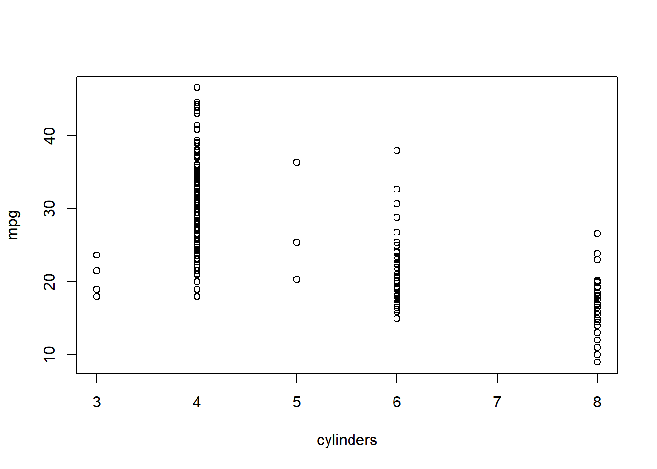
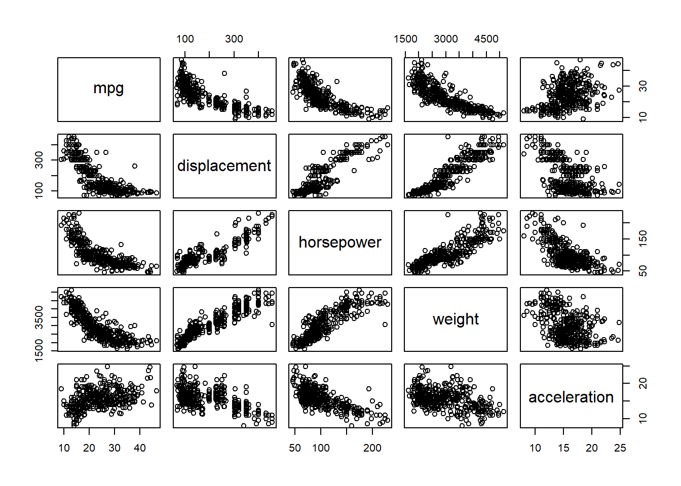
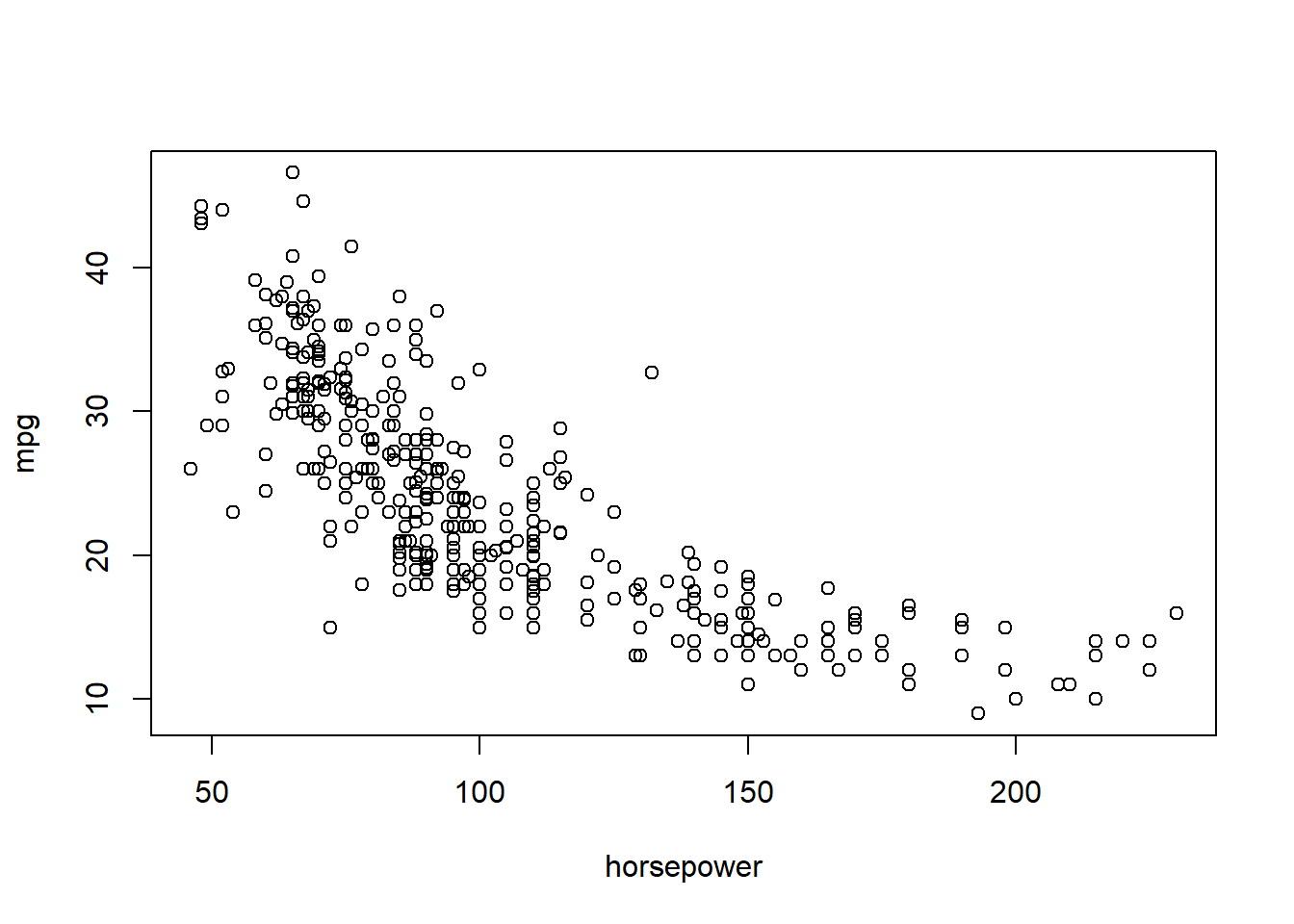
Auto=read.table("https://raw.githubusercontent.com/karlho/knowledgemining/gh-pages/data/Auto.data")# fix(Auto) # Starting the X11 R data editor#If you run fix it allows you to interactively edit data. You can edit the data from the data frame.# Auto=read.table("https://raw.githubusercontent.com/karlho/knowledgemining/gh-pages/data/Auto.data",header=T,na.strings="?")# fix(Auto)Auto=read.csv("https://raw.githubusercontent.com/karlho/knowledgemining/gh-pages/data/Auto.csv",header=T,na.strings="?")# fix(Auto)dim(Auto)
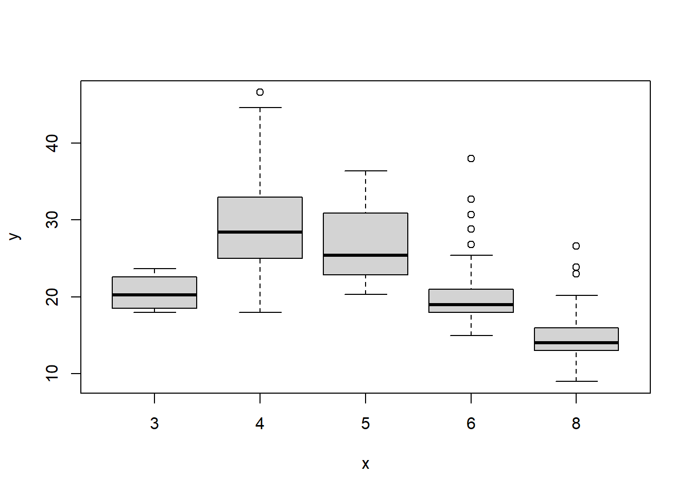
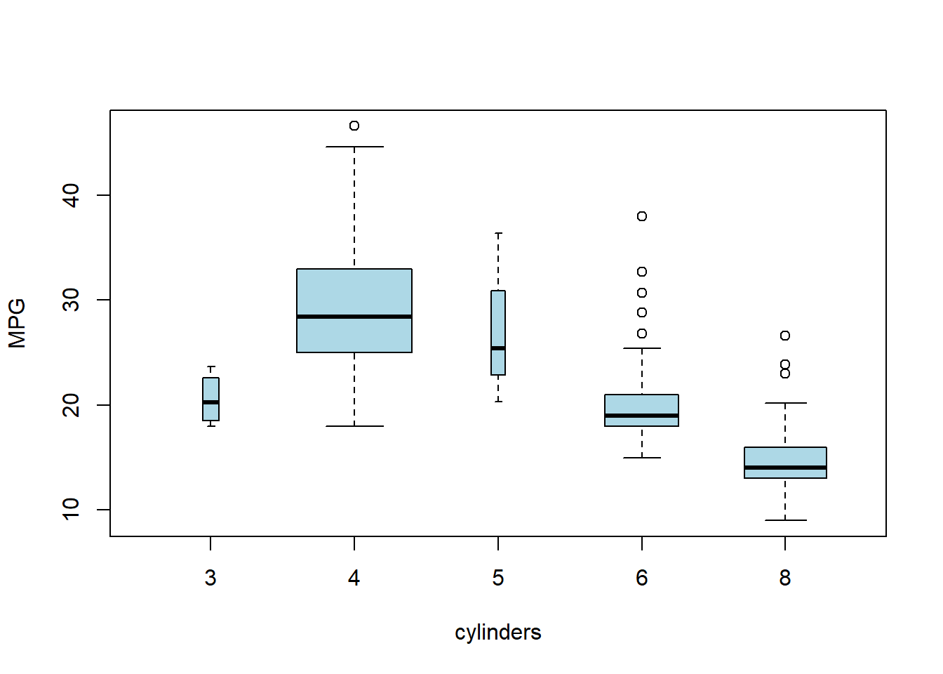
# identify(horsepower,mpg,name) # Interactive: point and click the dot to identify casessummary(Auto)
      mpg          cylinders      displacement     horsepower        weight
 Min.   : 9.00   Min.   :3.000   Min.   : 68.0   Min.   : 46.0   Min.   :1613
 1st Qu.:17.50   1st Qu.:4.000   1st Qu.:104.0   1st Qu.: 75.0   1st Qu.:2223
 Median :23.00   Median :4.000   Median :146.0   Median : 93.5   Median :2800
 Mean   :23.52   Mean   :5.458   Mean   :193.5   Mean   :104.5   Mean   :2970
 3rd Qu.:29.00   3rd Qu.:8.000   3rd Qu.:262.0   3rd Qu.:126.0   3rd Qu.:3609
 Max.   :46.60   Max.   :8.000   Max.   :455.0   Max.   :230.0   Max.   :5140
                                                 NA's   :5
  acceleration        year           origin          name
 Min.   : 8.00   Min.   :70.00   Min.   :1.000   Length:397
 1st Qu.:13.80   1st Qu.:73.00   1st Qu.:1.000   Class :character
 Median :15.50   Median :76.00   Median :1.000   Mode  :character
 Mean   :15.56   Mean   :75.99   Mean   :1.574
 3rd Qu.:17.10   3rd Qu.:79.00   3rd Qu.:2.000
 Max.   :24.80   Max.   :82.00   Max.   :3.000
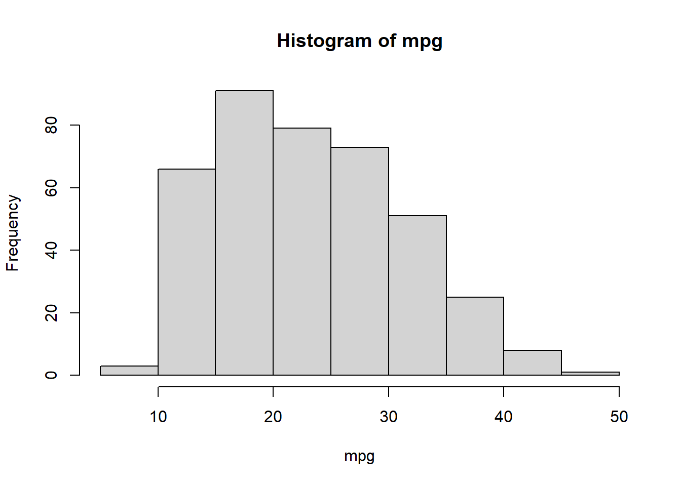
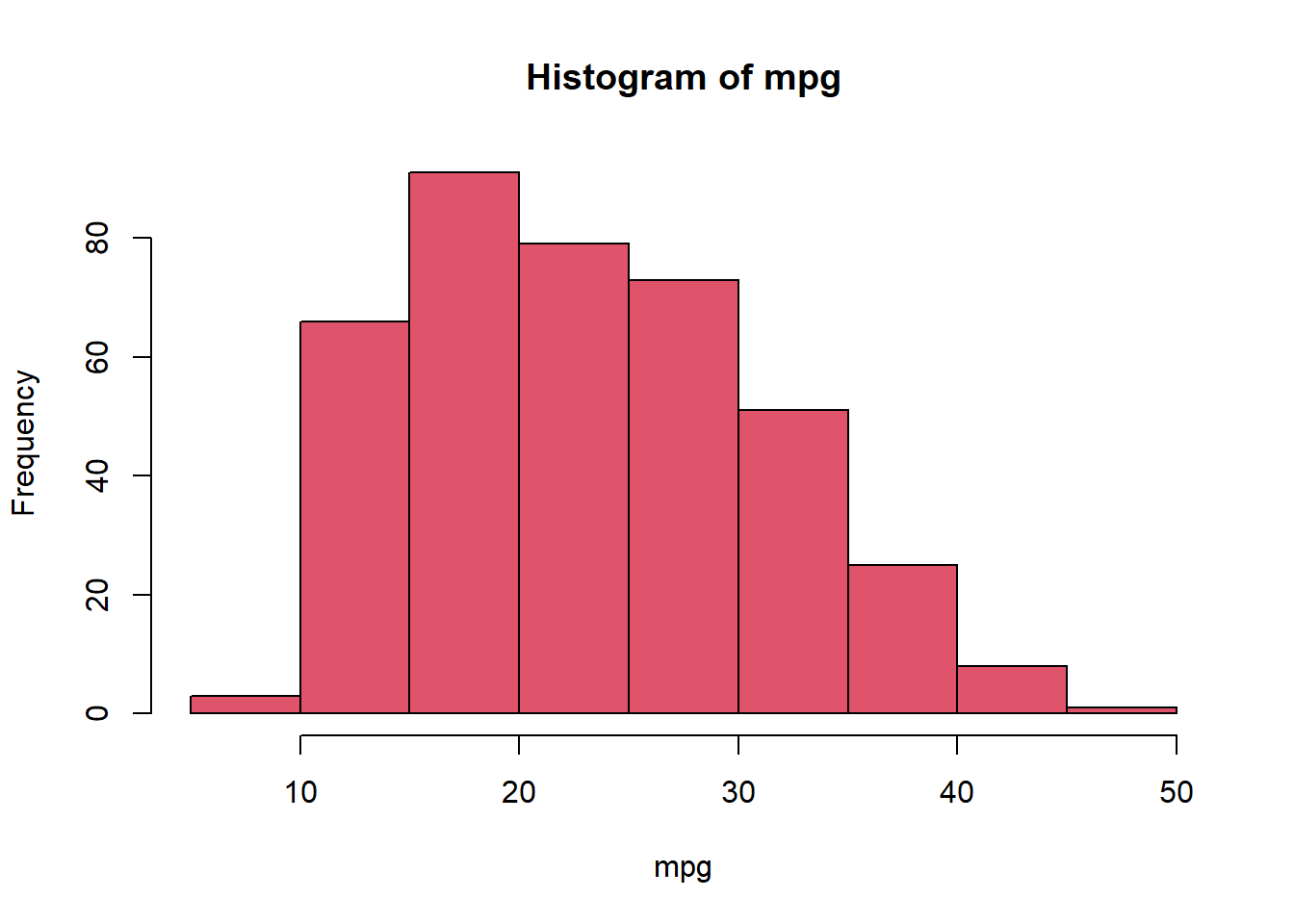
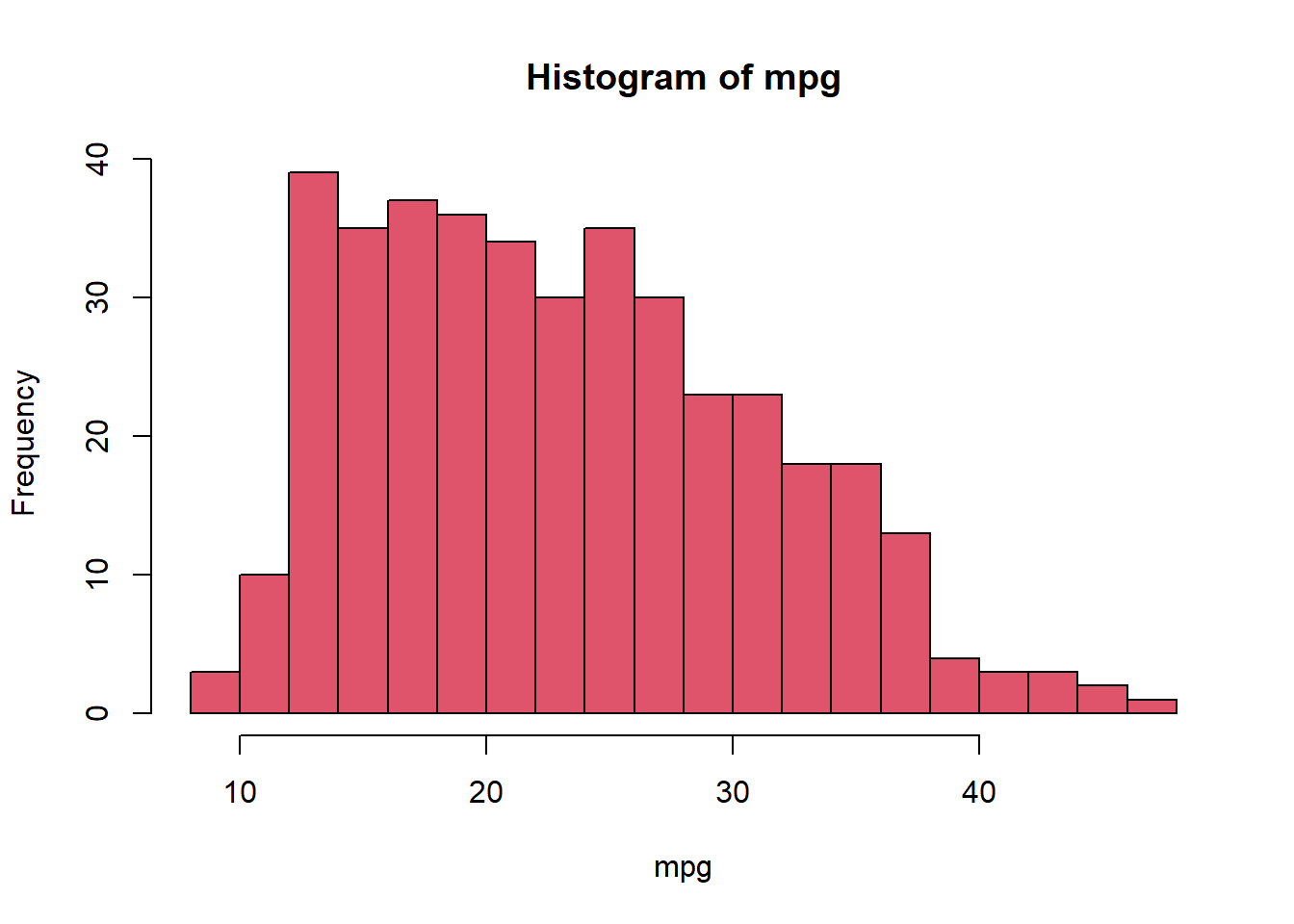
summary(mpg)
   Min. 1st Qu.  Median    Mean 3rd Qu.    Max.
   9.00   17.50   23.00   23.52   29.00   46.60
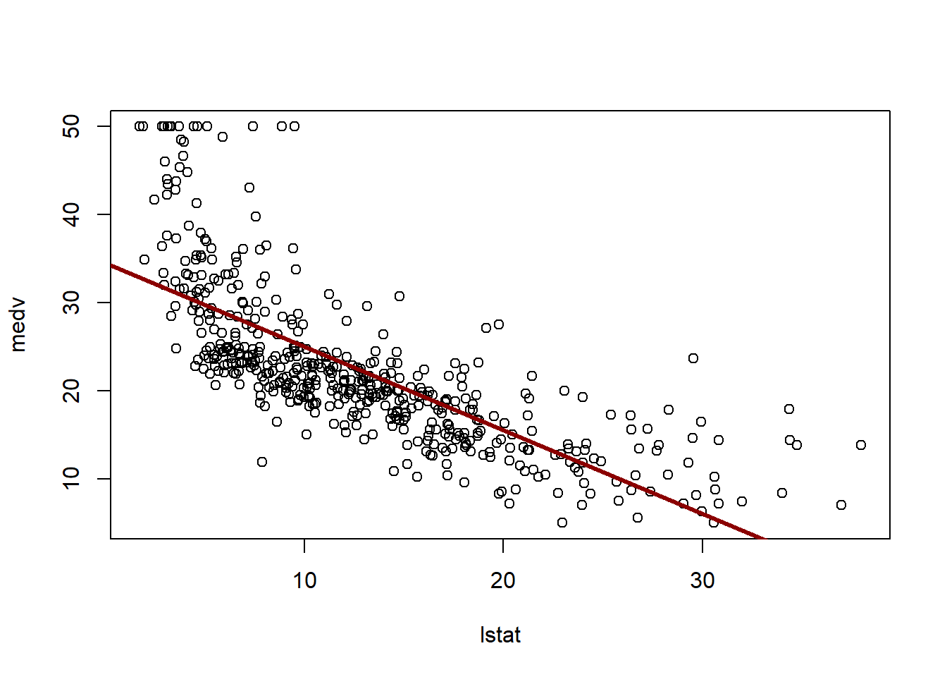
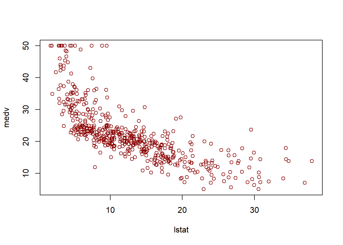
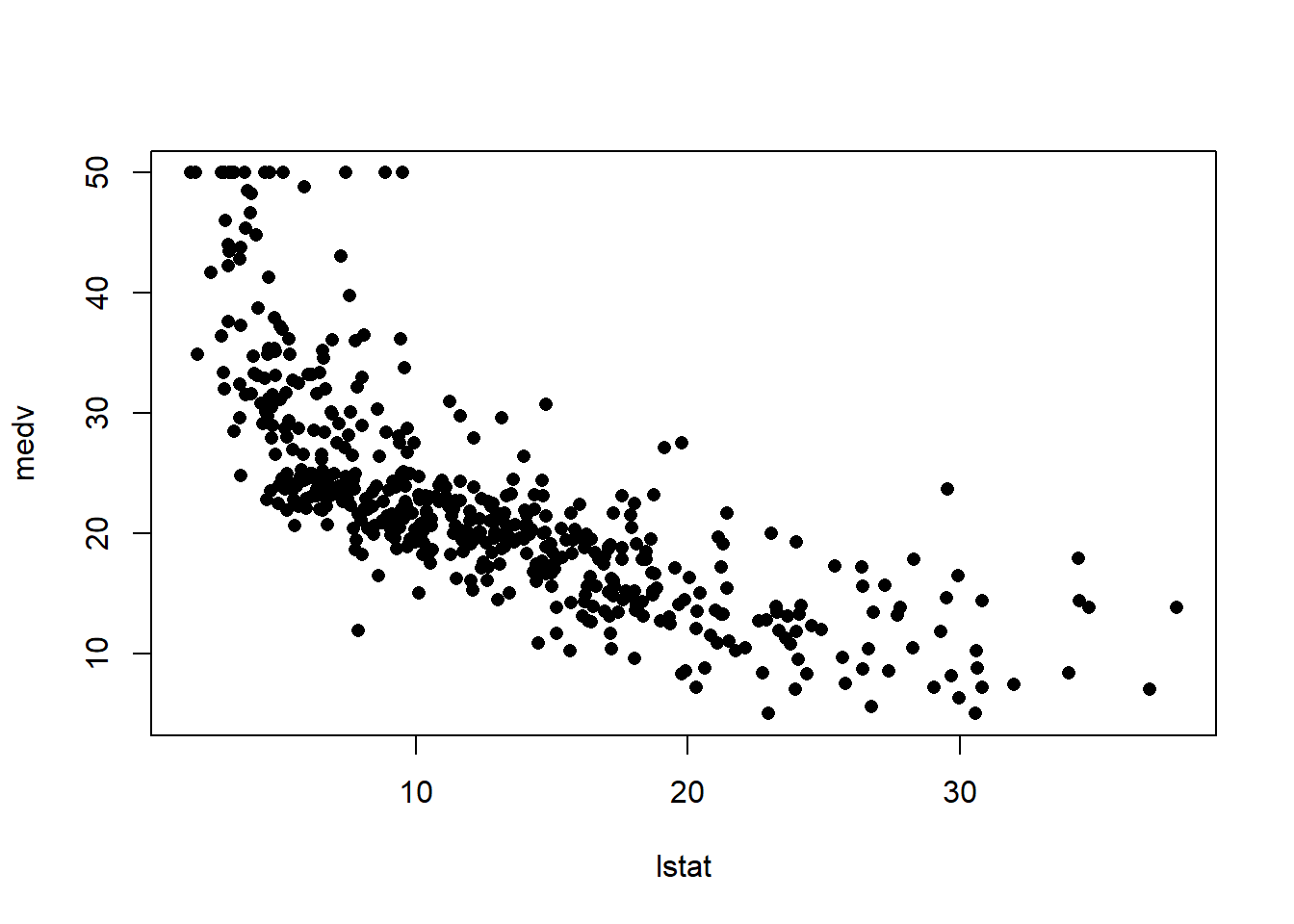
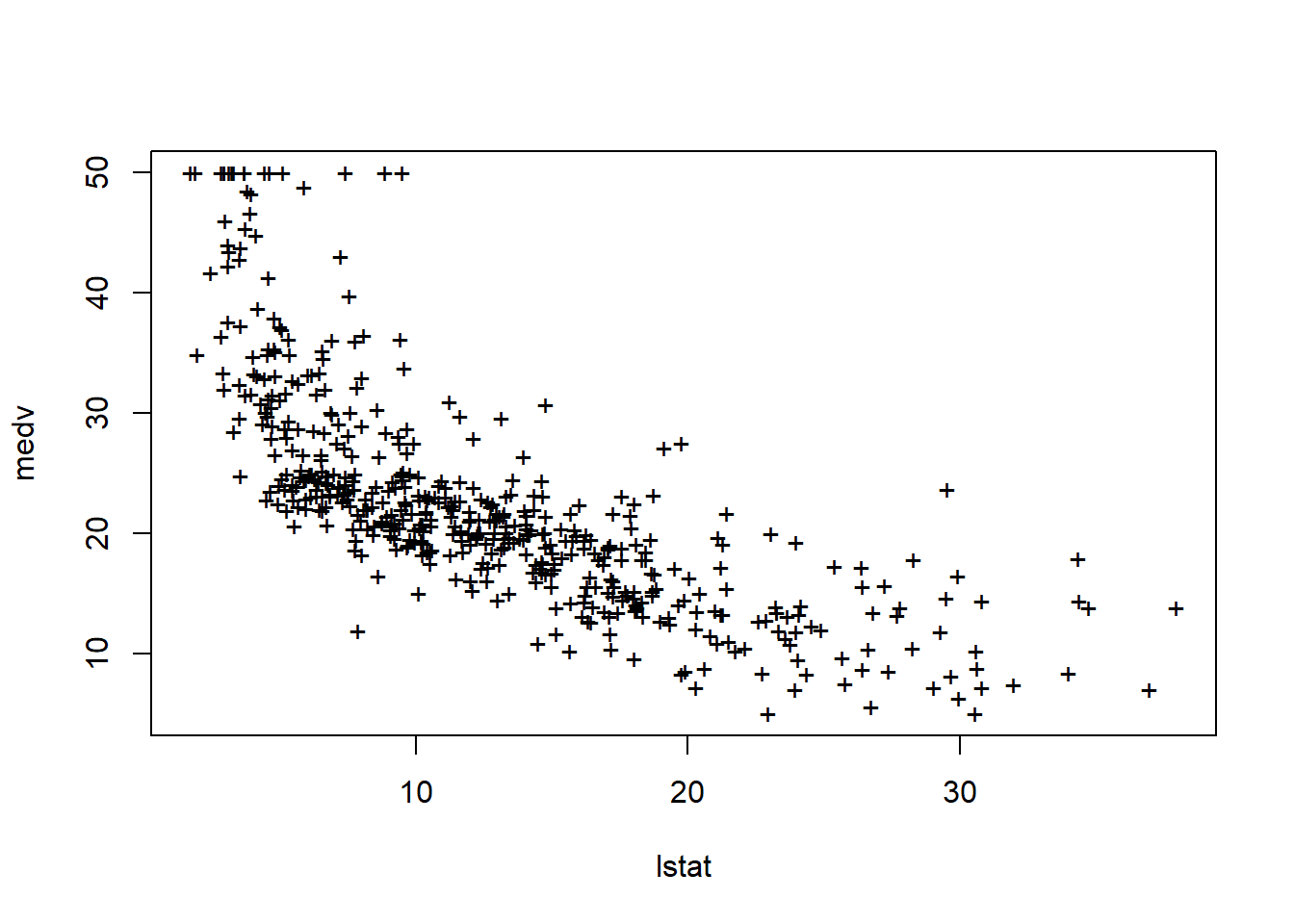
# What is the difference between "conference" and "prediction" difference?plot(lstat,medv)abline(lm.fit)abline(lm.fit,lwd=3)abline(lm.fit,lwd=3,col="darkred")
Interaction Terms (interactions and single effects
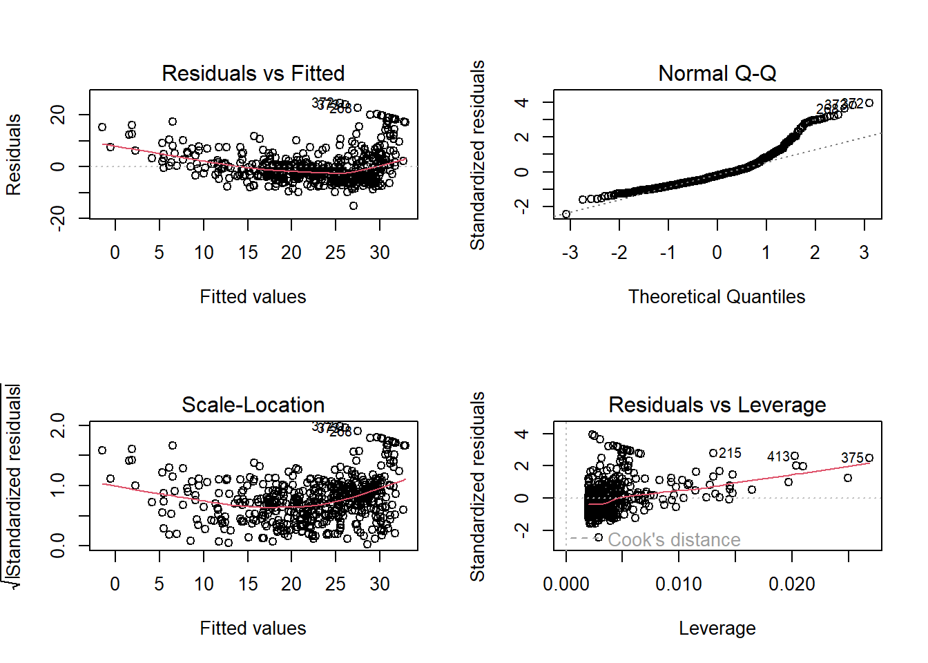
summary(lm(medv~lstat*age,data=Boston))
Call:
lm(formula = medv ~ lstat * age, data = Boston)

Residuals:
    Min      1Q  Median      3Q     Max
-15.806  -4.045  -1.333   2.085  27.552

Coefficients:
              Estimate Std. Error t value Pr(>|t|)
(Intercept) 36.0885359  1.4698355  24.553  < 2e-16 ***
lstat       -1.3921168  0.1674555  -8.313 8.78e-16 ***
age         -0.0007209  0.0198792  -0.036   0.9711
lstat:age    0.0041560  0.0018518   2.244   0.0252 *
---
Signif. codes:  0 '***' 0.001 '**' 0.01 '*' 0.05 '.' 0.1 ' ' 1

Residual standard error: 6.149 on 502 degrees of freedom
Multiple R-squared:  0.5557,    Adjusted R-squared:  0.5531
F-statistic: 209.3 on 3 and 502 DF,  p-value: < 2.2e-16
----------
Assignment 2
TEDS_2016 <-read_dta('https://github.com/datageneration/home/blob/master/DataProgramming/data/TEDS_2016.dta?raw=true') #Note read_stata does not work with this version of R. Need to utilize haven library and "read_data" with apostrophe and not quotation marks around link.
Question: What problems do I encounter with dataset?
Answer: There are a significant number of missing values in the form of NA in the dataset. It is also unclear if the “0” values are true 0 or if they are a different way of indicating a missing value.
Question: How to deal with missing values?
Answer: There are several methods to address missing data in a dataset.
Listwise deletion: Removing the entire row of data to not include in the analysis if there are any missing values in that row. We could first detect missingness through a visualization to understand the impact listwise deletion could have on our data. If the missing values are not random and if they reduce our sample size substantially, this is likely to impact the strength of findings and using the dataset.
Best guess imputation.
Multiple imputation.
Aggregate: If there is structure to the data, then we can aggregate so missing values do not have such an impact. For example, we could move from monthly to yearly.
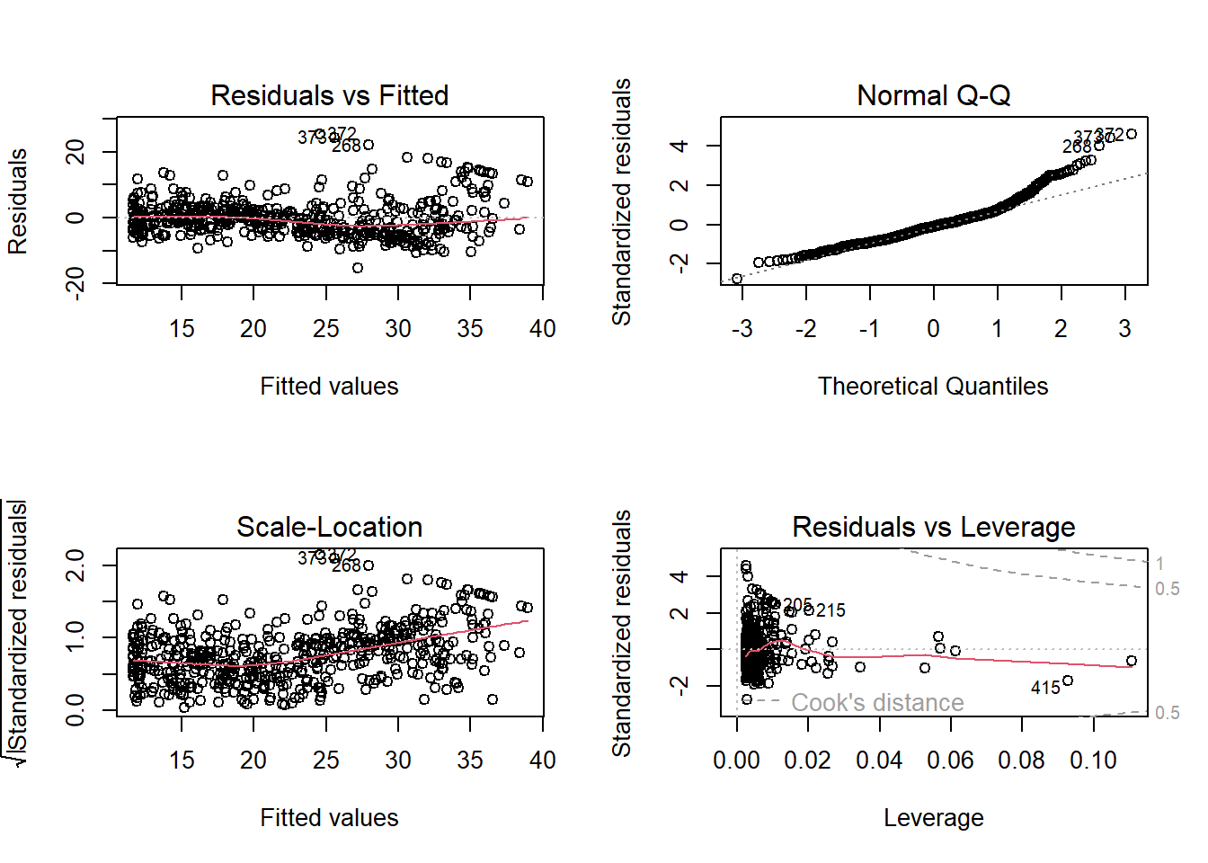
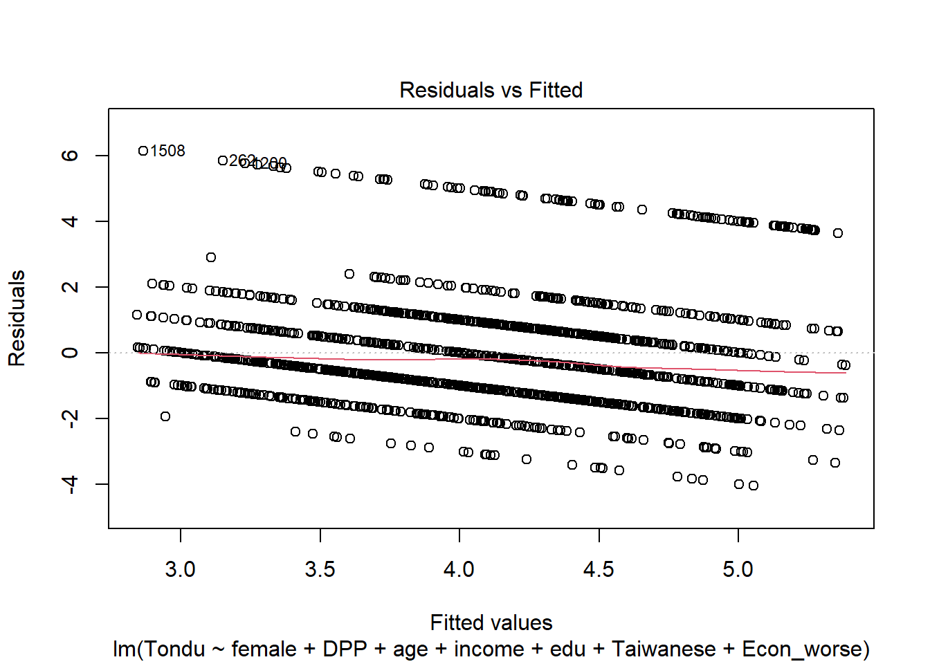
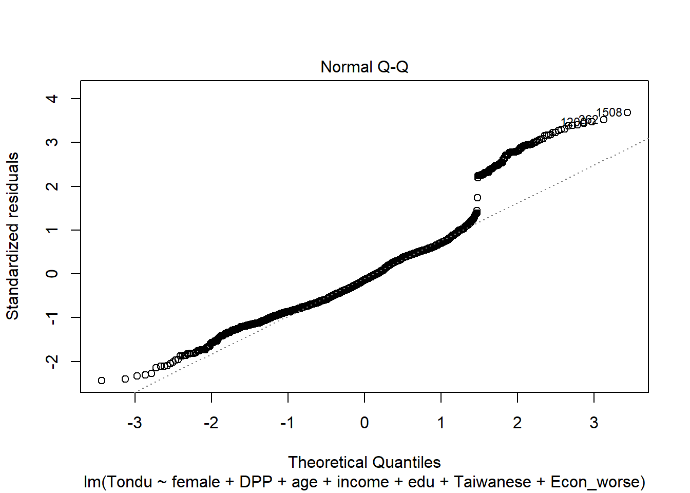
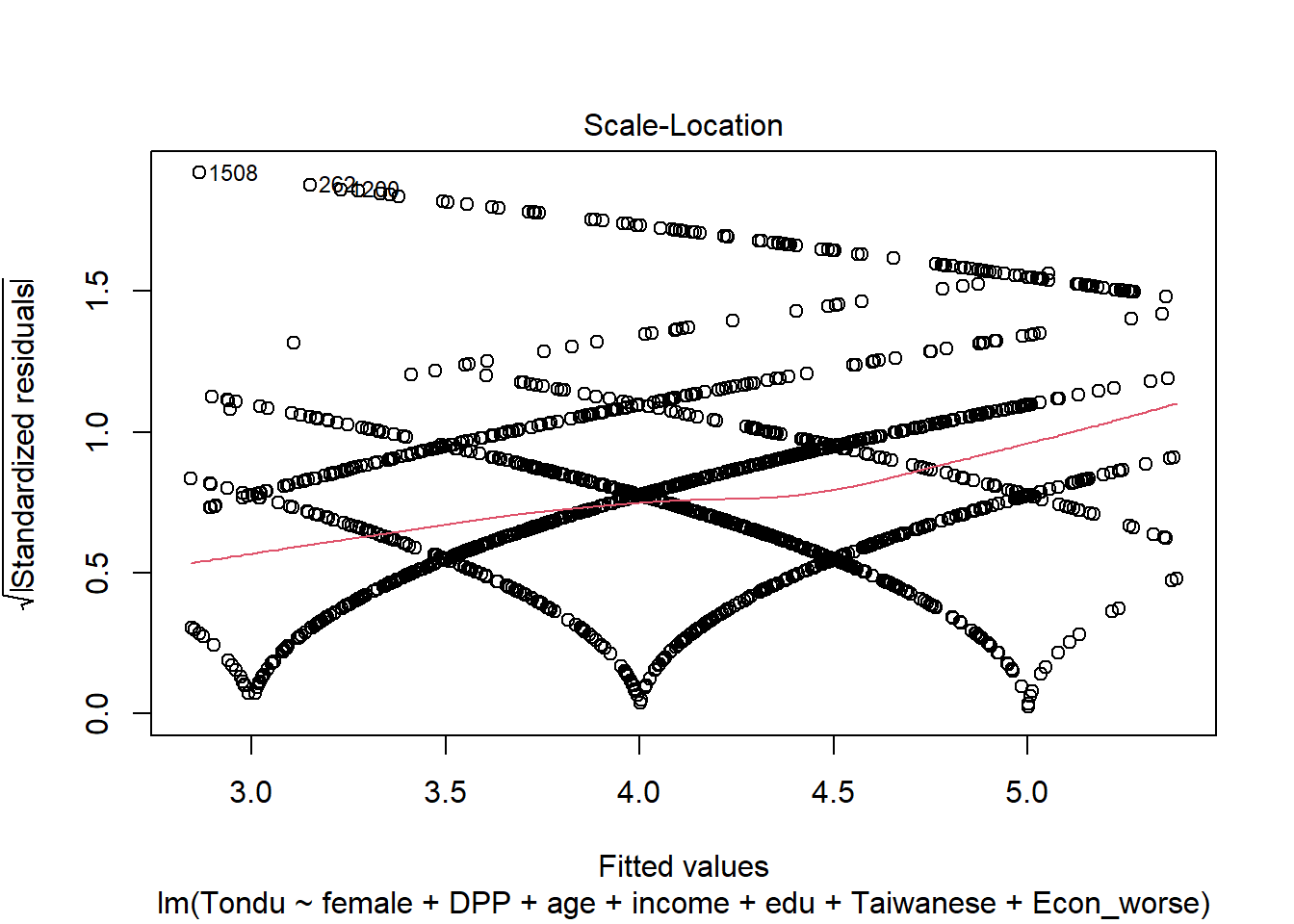
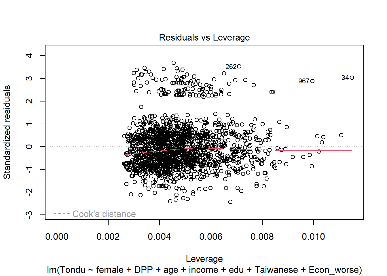
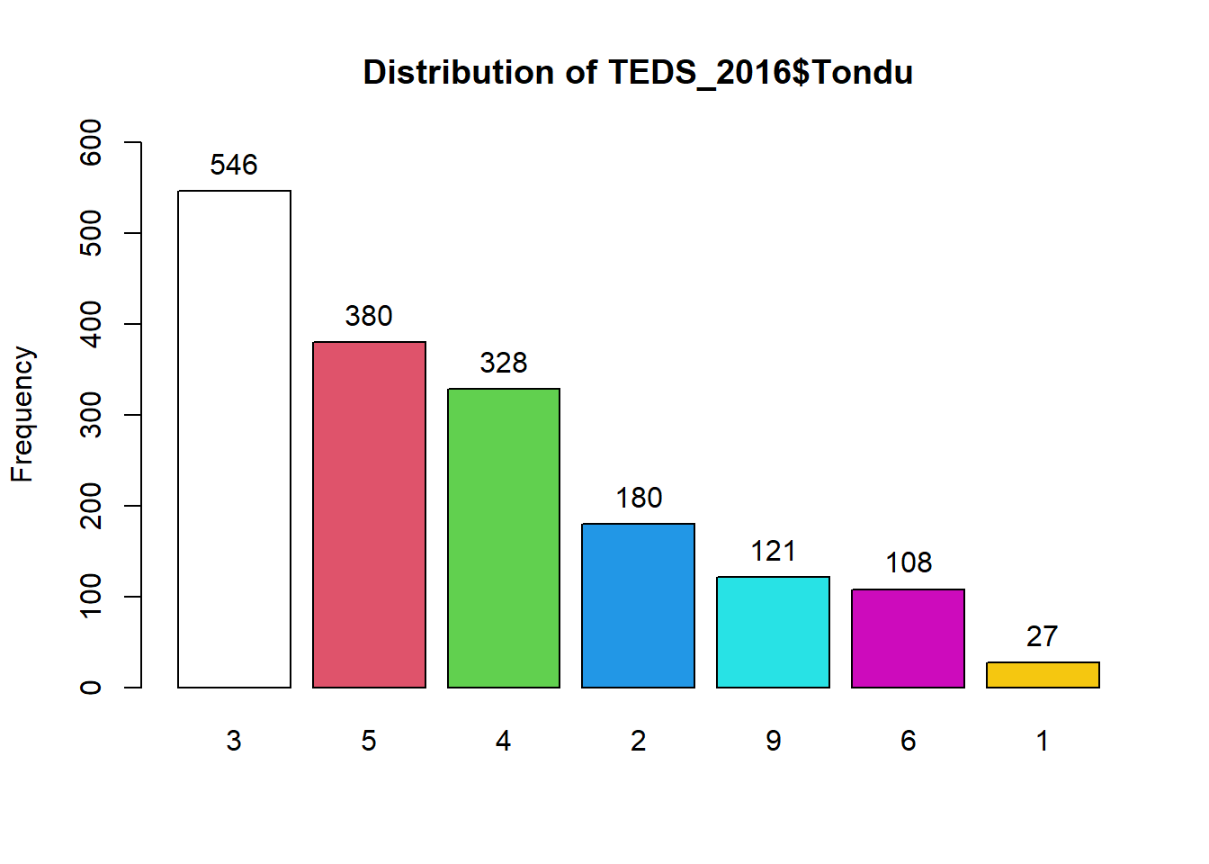
Explore Relationship between Tondu and other variables